Fitting of Straight Line
Robust fitting of a stright line
One from most trivial problems of statistical regression analysis is fitting of a straight line. I selected this well-known problem to illustrate
- usage of Minpack library to least square fitting by the least square method (LS) together with
- usage of robust statistical methods and also to prepare
- a simple reference example for testing of any software.
All required code can be found in the archive. Please read README for detailed description of included files.
Reference Data and Solution
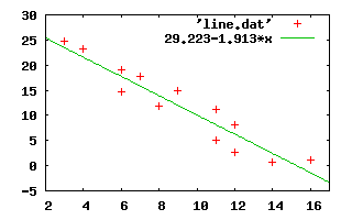
As data for a working example, I selected a tabulated values for a straight line from excellent mathematical handbook: Survey of Applicable Mathematics by K. Rektorys et al. (ISBN 0-7923-0681-3, Kluwer Academic Publishers, 1994). The data set is included in the archive as line.dat. Normal equations:
 14*a +  125*b = 170
125*a + 1309*b = 1148.78
and LS solution:
a   = 29.223
b   = -1.913
S0  = 82.6997
rms =  2.625
sa  =  1.827
sb  =  0.189
Using Minpack
Simple usage of Minpack in LS case is straightforward. One calls hybrd (Jacobian is approximated by numerical differences) or hybrj (must specify second derivatives) and one pass a subroutine to compute vector of residuals in a Minpack required point. Minpack uses Powell’s method which combines location of minimum with conjugate gradient method (locate minimum in direction of most steeper slope) far from minimum and Newton’s method (fit the function with multidimensional paraboloid and locate minimum by intersection of tangent plane with coordinate axis) near of minimum. For the straight line, we define a + b * xi and minimizing of sum for i = 1 to N: S = ∑ (a + b * xi - yi)² The vector for Minpack is ∂S/∂a = ∑ (a + b * xi - yi) ∂S/∂b = ∑ (a + b * xi - yi)*xi. The Jacobian is than
∂²S/∂a²    ∂²S/∂a∂b
∂²S/∂b∂a   ∂²S/∂b²
or
N ∑ xi ∑ xi ∑ xi²
All the sums can be found in minfunj in straightlinej.f90. The call of hybrj search for a minimum of the function. On output, the located minimum is included in fvec and I added a code to compute covariance matrix to estimate statistical deviations of parameters and their correlation. With gfortran I get the solution on 64bit machine:
...
minfun: par =   29.22344    -1.91302  sum =  82.68976
minfun: par =   29.22344    -1.91302  sum =  82.68976
hybrj finished with code           1
Exit for:
algorithm estimates that the relative error between x and the solution is at most tol.
qr factorized jacobian in minimum:
q:

0.10769513068469699       0.99418396628934158
-0.99418396628934158       0.10769513068469688

r:
152.97596122677001        1371.8039727109779
1371.8039727109779        17.656368881644468

inverse of r (cov):

0.25799238244686612      -2.87651125847342495E-002
-2.87651125847342495E-002  3.20772561895261684E-003

covariance:

1.7777772679919355      -0.19821501231688973
-0.19821501231688973      2.21038374592466315E-002

No. of data = 14
solution = 29.223435764531654 -1.9130248056275454
with dev = 1.3333331421636287 0.14867359368511487
residual sum = 82.689756238430220
rms = 2.6250358130641160
The results must correspond (within precision of tree digits) to the reference solution. As we can see, there is a great discrepancy in deviations of parameters. The Minpack’s estimation is little bit optimistic. I think that is due to difference between matrix inversion (which is usually used) and Minpack’s covariance estimation. On the other side, the values are the same from practical point of view.
Just for information. The inverse matrix (all by Octave) of Jacobian in minimum is (inv(.))
 0.4846353  -0.0462792
-0.0462792   0.0051833
and the QR factorization ([q,r,.]=qr(.)):
q =
-0.995472   0.095060
-0.095060  -0.995472

r =
-2.0541e+00 -1.2576e+02
0.0000e+00  -1.3150e+03
The Q matrix columns are base vectors (eigenvectors) of solution (the principal axes of covariance ellipsoid) and the diagonal elements are estimates of eigenvalues values (major and minor semiaxes of the ellipse) [l,v]=eig(.).
l =
-0.995457   0.095208
0.095208   0.995457

v =
2.0447e+00   0.0000e+00
0.0000e+00   1.3210e+03
The second supplied routine straightline.f90 does the same work but without explicit knowledge of the second derivatives. The Jacobian is estimated by numerical differences.
The solution can be also done via lmdef, lmder routines in Minpack. It is equivalent to presented solution but doesn’t offers generalization toward robust methods.
Robust Fitting
The reference robust fitting procedure is included in rstraightline.f90.
The fitting is logically divided onto two parts. The first part implements minimizing of sum of absolute deviations to get robust estimation of proper solution and MAD (mean of absolute deviations). There is little change with respect on LS because minimizing function have no derivation in minimum. We need another method without using of derivatives. I’m using code prepared by John Burkardt, namely using Nelder-Mead Minimization Algorithm (simplex method). I slightly rearranged the code to nelmin.f90.
The resultant parameters are used to obtain MAD by looking for its median by a quick way algorithm described in Niklaus Wirth’s Algorithms + Data Structures = Programs. The solution is than passed as start point for hybrd which is the second part. The minfun is similar to non-robust version. Only difference between predicted and computed solution (residual) is not directly used, but a cut-off function is used (Tukey’s function). This small change does robust fitting itself.
.....
medfun: par=   30.57930  -1.918842   sum=   29.9467137
medfun: par=   30.57930  -1.920842   sum=   29.9506577
ifault=           0   29.940157123526994
t=   30.579306941153348       -1.9198428764730142
4.3939266204833984        2.9615066
minfun: par =  30.57931  -1.91984   sum =  106.17691
.....

minfun: par =  29.24548  -1.91425   sum =   82.69177
hybrd finished with code:           1
Exit for:
algorithm estimates that the relative error between x and the solution is at most tol.
qr factorized jacobian in minimum:
q:

-0.10942034931424138      -0.99399556696996860
0.99399556696996860      -0.10942034931424133

r:

29.315789045435952        295.17538616058539
295.17538616058539           4.3667770003656630

inverse:

5.3177769129754946      -0.52802747846866527
-0.52802747846866527      5.24418460845494372E-002

covariance:

2.7756865626932967      -0.27561118127052436
-0.27561118127052436      2.73727405045027551E-002

No. of data = 14
solution = 29.245477844988198 -1.9142493591979692
with dev = 1.6660391840209812 0.16544709276533920
residual sum = 82.691772460937500
rms = 2.6250678159642766
The output values are practically the same as in non-robust case. Only the difference is estimation of parameter’s deviation. I’m using the formula recommended by Hubber(1980), eq. (6.6) p. 173. The real power of the robust fitting can be easy demonstrated by adding any outlier (point with really different value) to the set, for example, a point with coordinate 10,100. Try to see the robust algorithm in action. It should be practically the same while non-robust solution gives some strange values.
Minpack Fortran Interface
The original Minpack is written in Fortran 77. I’m using modern Fortran (Fortran 90, 95 or 2003) which supports better type checking via interfaces. I prepared such interface which is included in Archive as minpack.f90 and must be passed to compiler during compilation. The module did not changed original API to Minpack routines to prevent any programming errors. So you also must pass to the routines “working arrays” (wa). One is used in modern Fortran more elegant way as automatic arrays (arrays allocated automatically when subroutine is entered and deallocatedon its exit).
Estimation of an initial solution
The solution will not depend on starting point only in linear case. Every complex real) case will lead to non-linear solution with a lot of local minimums which will attract the simplex or the gradient (Powell’s method) to a “wrong” solution. To locate global minimum (eg. required solution), I recommends use of genetic algorithms as predictors of a global minimum. The genetic algorithms will locate right minimum with a low precision and we can use some modification of above codes to determine the minimum with required precision.